 Plotting different performance metrics against the number of trees in random forest. Source
I came across the following paper during my Masters coursework that addresses a practical issue in the use of the random forest model, and in general, any other bootstrap aggregating ensembles:
1. Motivation
This is an interesting paper as it directly addresses a fundamental question on whether the number of base learners in a bagging ensemble should be tuned. In the case of random forest (RF), the number of trees T is often regarded as a hyperparameter, in the sense that either too high or too low of a value would yield sub-par model performance. Tuning of T is typically done by plotting the one or multiple chosen out-of-bag (OOB) metrics, such as the error rate, as a function of T:
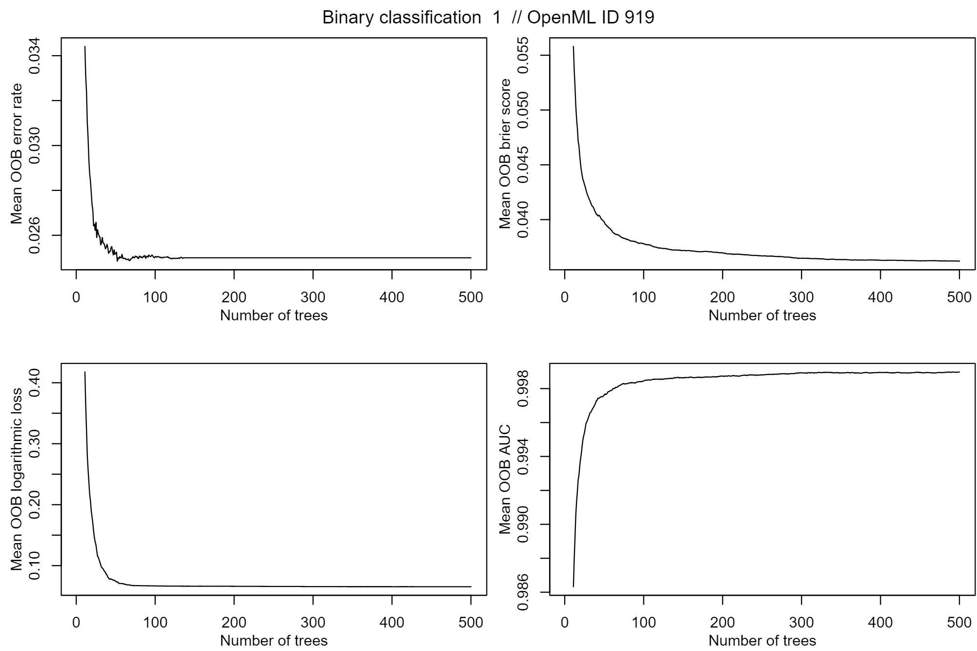 Different OOB metrics (error rate, Brier score, log loss, AUC) as a function of T. Source
In the case above, there are clear indications of convergence in T, and any further increase in T brings either marginal or zero improvements in model performance. However, that's not always the case, prompting the treatment of T as a model hyperparameter:
 Non-convergence of T. Source
2. Objectives of paper
Based on this motivation, the authors move step by the step to give this issue a structured treatment along the following objectives:
| Quoted from abstract | Layman explanations |
| (i) Provide theoretical results showing that the expected error rate may be a non-monotonous function of T, and explaining under which circumstances this happens | Show that the error rate of RF may increase or decrease as T increases (non-monotonous), depending on a certain phenomenon that could be observed from the testing dataset. |
| (ii) Provide theoretical results showing that such non-monotonous patterns cannot be observed for other performance measures such as the Brier score and the log loss (for classification) and the MSE (for regression) | Show that such non-monotonicity cannot be observed for performance metrics such as the Brier score, log loss and MSE, even though it can be observed for the error rate - sorry for the double negative, take a moment to digest that before you get confused further. (It is also shown in the paper that the ROC-AUC follows such non-monotonicity.) |
| (iii) Illustrate the extent of the problem through an application to a large number (306) datasets | Validate findings via empirical experimentations using public ML datasets |
| (iv) Argue in favor of setting T to a computationally feasible large number as long as classical error measures based on average loss are considered | Conclude that T should not be tuned, but set to a feasibly large number. |
3. Structure of paper
- Motivation and literature review
- Build up RF and various performance metrics for theoretical context
- Theoretical treatment (mainly binary classification, results for multiclass classification and regression are extrapolated and inferred)
- Empirical validation
- Conclusions and extensions
4. Five takeaways from the authors
Without boring you as the reader on the specifics of the theoretical and empirical treatments to the problem, here are the key takeaways from the authors (with my translations):
- Non-monotonicity (as a function of T) can only be observed for the error rate and the ROC-AUC, but not for typical performance metrics such as the Brier score, log loss, or MSE.
- *The behaviour of the error rate as a function of T (error rate curve) is largely dependent on the empirical OOB distributions of the prediction errors εi - this is the most important point in this paper for me, to be elaborated further.
- For regression, non-monotonicity can be observed from median-based (as opposed to mean-based) performance metrics. This makes sense since typical recursive partitioning in the base learners goes for squared error minimization.
- The biggest OOB performance gain comes from the first 250 trees; going from 250 to 2000 trees yields minimal performance gains. This is true for binary classification, multiclass classification, and regression.
- More trees are better - non-monotonicity is only observed under specific conditions, with specific performance metrics. Even under non-monotonicity, the difference between the converged metric and its global extreme is minimal. Therefore, set T to a computationally feasible large number.
5. Empirical OOB distributions of prediction errors
One of the key takeaways from this paper is that the behaviour of the error rate as a function of T (error rate curve) is largely dependent on the empirical OOB distributions of the prediction errors εi. In the paper, it was shown theoretically that the convergence rate of the error rate curve is only dependent on the distribution of εi. In particular,
- In a largely accurate (many observations with εi ≈ 0, few observations with εi ≈ 1) ensemble, observations with εi > 0.5 will be compensated by observations with εi < 0.5 , in such a way that the error rate curve is monotonously decreasing.
- However, in ensembles with many εi ≈ 0 and a few εi ≥ 0.5 that are close to 0.5, a problem arises. By the authors' computations, due to these fringe cases (model is uncertain ∴ εi ≈ 0.5), the error rate curve falls down quickly, then grows again slowly to convergence. The following should make a convincing case:
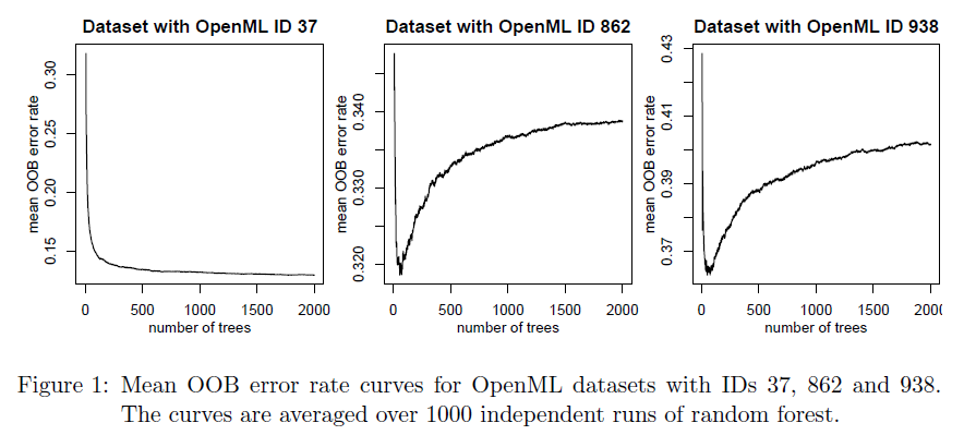 OOB error rate curves for three datasets from OpenML. Source
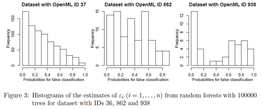 OOB εi distributions from RF models on the same three datasets. Source
These are rather high impact findings as in practice, the empirical OOB distributions of εi are often not reviewed, especially in the setting of RF or any other ensemble modeling exercise. (On the other hand, if your training is in statistics, then linear regression diagnostics should be very familiar. Just sayin'.)
6. Practical implications from this paper
Finally, all that talk for what we can do in practice:
- As part of model maintenance, check on the distribution of εi. When concept drift kicks in in the future, your model could become doubly misspecified - one count from training-testing data disparity and one count on the selection of T. Also notice that the distribution of εi is a function of e.g. size of the dataset (both n and p). This should be intuitive.
- Understand the behavior of your selected performance metric as a function of T. To give a naive example, optimizing ROC-AUC vs. optimizing log loss with respect to T should now be very different to you.
- Finally, under normal or slightly perturbed conditions (again on
distribution of εi) , a large T is still better.